Recursion and Backtracking are important problem solving approaches. Recursion may also be called as the alternative to our regular iterative approach of solving any problem. Recursion provides us with an elegant way to solve complex problems, by breaking them down into smaller problems and with fewer lines of code than iteration. However, not every recursive solution is better than an iterative one. Backtracking too employs recursion to solve complicated problems, which involving possiblities of multiple solutions.
The following tutorial will allow you to gain an in-depth knowledge of the concepts, implementations, and usage of recursion and backtracking. With that, let’s get started!
Scope
We will delve deeply into the following topics in this tutorial, with examples to enhance our understanding
- What is recursion?
- When should we use Recursion?
- Format of recursive function
- Base condition in recursion
- Example
- What is backtracking
- Difference between recursion and backtracking
- Backtracking algorithm
- Example of recursion & backtracking
- Application of recursion & backtracking
Takeaways
Backtracking uses recursion to solve it’s problems. It does so by exploring all the possiblities of any problem, unless it finds the best and feasible solution to it.Recursion occurs when a function calls itself repeatedly to split a problem into smaller sub-problems, until it reaches the base case.
Introduction
Have you ever been in a barber shop, where you seat in the middle of shiny mirrors, one placed in front of you and another behind you? There you see your image, within your image, within your image and so forth This is the recursive view of images where you can see countless images of yourself. This is the example of recursion.
However, this is recursion without a terminating case, because you cannot find a point where those images come to an end. They are just countless.
The word recursion derives from the word “recur”, and it means to occur, or appear, again.
Now, let us see what exactly recursion is.
What is Recursion?
Recursion is a programming pattern that is useful when a task can easily be split up into several similar, but simpler tasks. Or when a task can be simplified into an easy action plus a simpler variant of the same task.
Recursion can be defined as the process in which a function calls itself, either directly or indirectly. In simple terms, when a function calls itself, it is known as recursion. The function that is calling itself is called the recursive function.
For example, imagine an onion in your mind. Imagine you are peeling off just the outer layer of that onion. Now what do you see? Do you see another onion, only smaller? In your mind, you have looked into an onion and have seen a smaller onion; you have seen the recursive structure of onions— onions within onions.
A simple example —
function a()
  print("Hey, I'm a recursive function!")
  a()
Recursion involves a few important steps where the recursive methods play an important role. This is accomplished by breaking the whole problem into smaller problems. They then call individual copies of those smaller problems to solve them, simplifying the overall problem. The recursive call is the process of calling each copy of that smaller problem, one after the other, to solve it.(there may be multiple recursive calls).
But, there must be a terminating condition in recursion, otherwise this calls may go endlessly leading to an infinite loop of recursive calls and call stack overflow.
When should we use Recursion?
Have you ever wondered, how calling the same functions repeatedly may even be a use to you?
Sometimes we are unable to solve a problem iteratively due to it’s high complexity. But, if we break the problem into smaller versions of the problem, we may be able to find solutions for those smaller versions of the problem. And then, we may combine those solutions to arrive at our answer for the larger problem.
This exactly is the underlying concept behind recursion — Recursive functions break any problem up into smaller sub-problems, the answer to which is either already known or can be found by using another algorithm. Hence, finally combining the results to build up the answer for the entire problem.
We can use recursion for the following reasons:
Recursioncan be useful when dealing with problems that have many possible branches and are too complex for iteration.
For example, imagine you are searching for a file on your laptop. You enter the root folder, within that you enter another folder, and so forth as you climb folders on folders until you locate your file. You can think of it as a tree with multiple branches. So, these kinds of problems are best solved using recursion. For these types of problems, an iterative approach may not be preferable.
![]()
A recursive solution is usually shorter than an iterative one.
Let’s see how a recursive solution is usually more shorter(and simpler) compared to the iterative approach.
Suppose we want to compute the power of any number in JavaScript. Let’s go with the iterative approach.
function factorial(n){
    fact = 1;
    for(i = 1; i<=n; i++){
        fact = fact*i;
    }
    return fact;
}
alert(factorial(5))
If you go by the recursion approach, it is as simple as:
function factorial(n){
return (n<=1)? 1 : (n*factorial(n-1));
}
alert(factorial(5));
All recursive algorithms can [also] be implemented iteratively and vice versa.
Also, recursions are best suited and easiest for Trees and graphs to do traversal. There are several other usage of recursion, which we will discuss further in this article.
Format of recursive function
Whenever we are talking about recursive functions, we cannot deny the two most important parts of recursion
- A base case, in which the recursion can terminate and return the result immediately.
- A recursive case, in which the function is supposed to call itself, to break the current problem down into smaller problems
Similarly, the input size gets smaller and smaller with each recursive call, and we get the solution to that smaller problem. Later, we combine those results to find the solution to the entire problem.
This is a pattern followed by every recursive function. We can take the very popular example of the factorial function for this
function factorial(n):
if (n <= 1)  //Base Case
return 1;
else
return n * factorial(n-1); //Recursive Case
It can be well represented as:
                if n<=1 => return 1
               /
factorial(n) =
              \
               else   => return n * factorial(n - 1)
- If n <= 1, then everything is trivial. It is called the base case of recursion, because it immediately returns the result: factorial(1) = 1.
- Otherwise, we can represent factorial(n) as n factorial(n – 1) This is called a recursive step we transform the task into a simpler action (multiplication by n) and a simpler call of the same task (factorial with lower n). Next steps simplify it further and further until n reaches 1
The recursion tree for the above functionif called with factorial(3) will look like:
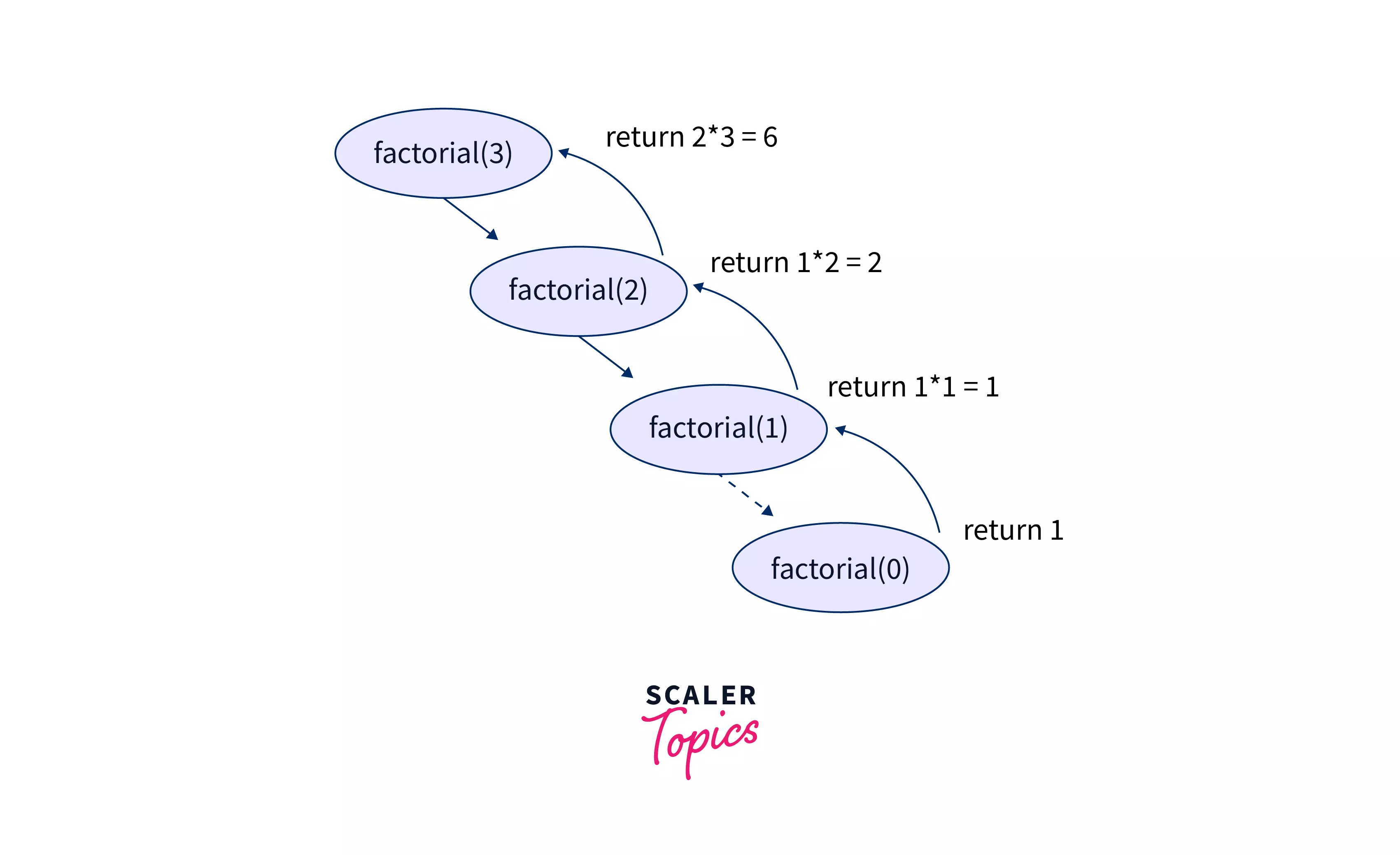
We will explain the recursion tree deeply in the upcoming examples.
Base condition in recursion
So, what exactly is a base case in recursion and why is it soo necessary? Well, the base case is the terminating case in recursion. This is where the recursive calls finally comes to an end, or terminate preventing any endless (infinite) recursive calls. It is a problem whose answer we already know and which can be directly returned without any further recursive calls being made. If base case is not provided, the entire memory can be exhausted by the infinite recursive calls, resulting in the call stack overflow.
Some note worthy points for the base condition in recursion are —
- While solving a recursive problem, we should always think does the recursive call make the problem smaller and approach the base case?
- Every recursive function must have one or more base cases depending on which the final answer is evauated.
Examples
Example 1: The classic example of recursion is calculating the factorial of any number. The factorial of any number is computed as the number multiplied by all the numbers below it till 1. Example: factorial of 4 (4!) = 4 * 3 * 2 * 1 So, it is something like –
factorial(n) = n * (n-1) * (n-2) * (n-3) * ... * 1
Or, factorial of any number n may be called as the number multiplied by the factorial of the number immediately below it
factorial(n) = n * factorial(n-1)
This forms our recursive case, since here, a function factorial will be calling itself passing a smaller version of problem as the parameter. So, you may assume this will be our code —
function factorial(n){
    return n * factorial(n-1)
}
But this code will simply crash, do you know why? Yes, obviously, we have not provided the base case! How would it ever know when to terminate? It will go on endlessly exhausting the entire memory, resulting in the call stack overflow. Base case is unavoidable. But, what should be the base case? Well, we already know the factorial of 0 or 1 is 1 0! = 1! = 1 and there is no factorial for negative numbers! So, we can simply have a check if the number is less than or equal to 1 then return 1. Then, our code becomes
function factorial(n){
    if(n<=1) //Base case
        return 1;
    else
        return n * factorial(n-1); //Recursive case
}
Suppose we want to calculate factorial(4) . It will be computed through the following steps —
- Firstly, it will call factorial(4) which checks the base condition if (n===0 or n===1), here n=4, which is neither 0 nor 1. So the condition fails and it goes to the else statement. There it will make a call to n * factorial(n-1) factorial(4) = 4 * factorial(3) //recursive case factorial(3) = 3 * factorial(2) factorial(2) = 2 * factorial(1) factorial(1) = 1 * factorial(0)
- Finally when factorial(0) will be called, it will reach the base case and return 1. The function will return, and while returning, it will calculate the value of all the smaller problems it broke into when it was calculating factorial.
The order of recursive calls can be depicted by a recursion tree shown below for factorial(4).
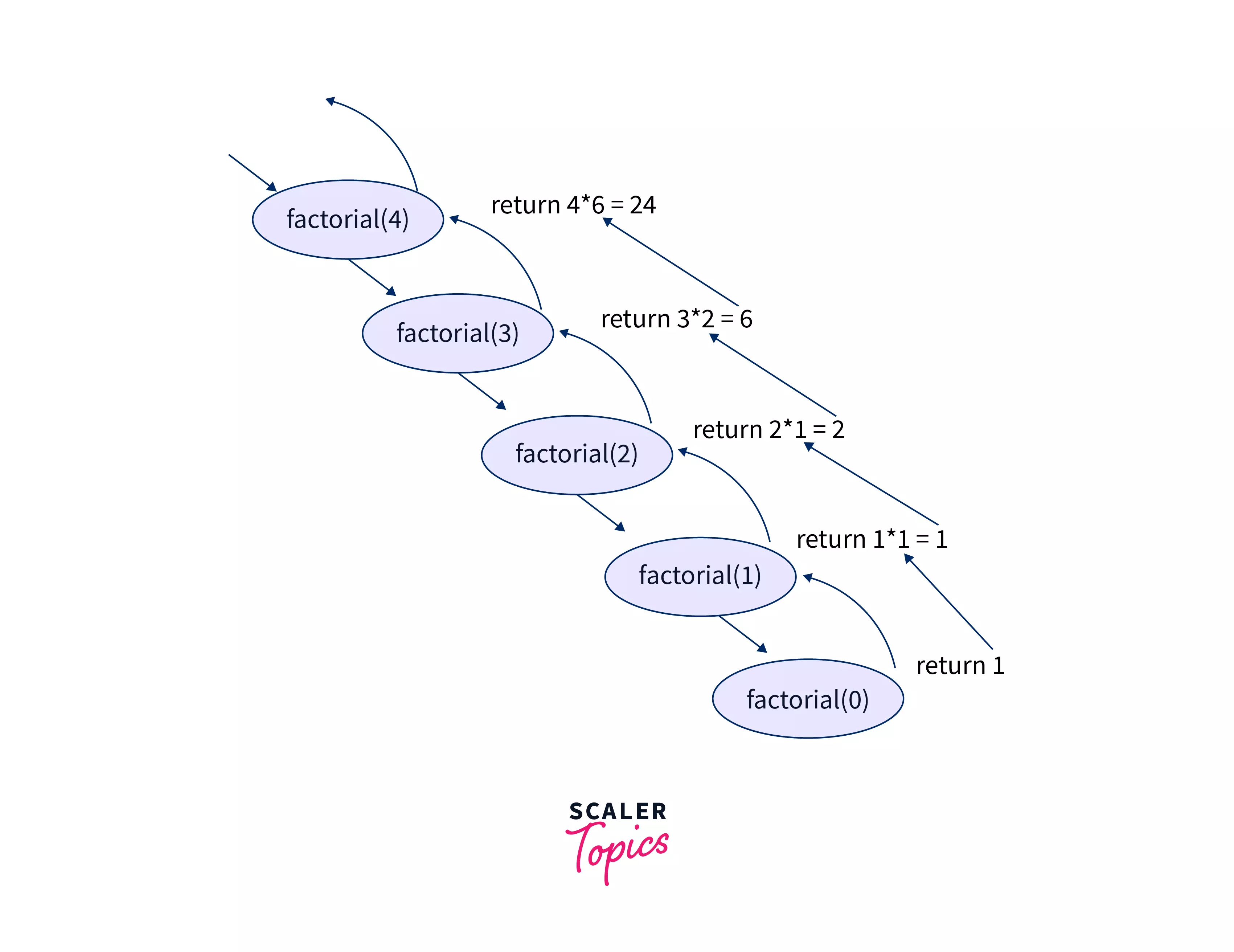
A recursion tree is a diagram of the function calls connected by pointed(up or down) arrows to depict the order in which the calls were made.
Example 2: Let us take one more example, calculating the fibonacci number using recursion. The Fibonacci numbers are the numbers in the following integer sequence 0, 1, 1, 2, 3, 5, 8, 13, 21, 34, 55, 89, 144,.. Here, each number is the sum of it’s previous and the 2nd previous number. In mathematical terms, the sequence Fn of Fibonacci numbers is defined by the recursive relation
Fn = Fn-1 + Fn-2
Here, Fibonacci(0) = 0 Fibonacci(1) = 1 These can be considered as our base case, since based upon these two, any n^th^ fibonacci number can be calculated. So, the code may be
function fibonacci(n){
if (n<=1) //Base case
    return n
else
    return fibonacci(n-1)+fibonacci(n-2) //Recursive function
}
The order of recursive calls can be depicted by a recursion tree shown below for fibonacci(5).
                           fib(5)
                       /             \
                     /                \
               fib(4)                fib(3)
             /        \              /       \
         fib(3)      fib(2)         fib(2)   fib(1)
        /    \       /    \        /      \
  fib(2)   fib(1)  fib(1) fib(0) fib(1) fib(0)
  /     \
fib(1) fib(0)
Note: Calculating fibonacci numbers using recursion is not a good approach though, since it takes exponential time to compute (beyond the scope of this article). However, this example is taken just for the sake of explanation.
Advantages/Disadvantages of Recursion
These are the advantages of recursion
- Usually code is simpler to write
- Extremely useful when a task can be simplified into an easy action plus a simpler variant of the same task.
- To solve problems which are naturally recursive for example – the tower of Hanoi.
- Recursion reduce the length of code.
- Useful in solving data structures – tree related problems.
Below are few disadvantages of recursion:
- Recursive functions are inefficient in terms of space and time complexity
- They may require a lot of memory space to hold intermediate results on the system’s stacks.
- Recursion can sometimes be slower than iteration because in addition to the loop content, it has to deal with the recursive call stack frame. This will result in more code being run, which will make it slower.
- The computer may run out of memory if the recursive calls are not properly checked(stack overflow), or the base case is not added.
- Sometimes they are hard to analyze or it is difficult understand the code.
Applications of Recursion
Recursive solutions are best suited to some problems. Below are a few examples —
- Tree Traversals
- Tree Problems: InOrder, PreOrder PostOrder
- Graph Traversals: DFS [Depth First Search] and BFS [Breadth First Search]
- Towers of Hanoi
- Backtracking Algorithms
- Divide and Conquer Algorithms
- Dynamic Programming Problems
- Merge Sort, Quick Sort
- Binary Search
- Fibonacci Series, Factorial, etc.
What is backtracking?
Think about a scenario where you are standing outside a maze, and you need to find the exit (see image). Now, you have a couple of ways you can try to find the exit door, uncertain of the outcome. You may either run into some wrong path, backtrack(move back to the starting point) and try to find a new path, or one in many chances, you may land into the correct path and reach your exit door. But out of multiple scenarios, you have only one path(marked in green) which will lead you to the exit door.
![]()
Basically, the idea is —
- we can build a solution step by step using recursion; e.g. In above example, we will try to find out multiple paths that can lead our desired exit door. And, we can travel into that path step by step using recursion.
- If during the process we realise that is not going to be a valid solution, then we stop computing that solution and we return back to the step before (backtrack).
Similarly, in programming, backtracking basically means that, if the current solution to your problem is not good or incorrect, you should eliminate it, move back (backtrack) and try another solution.
- Backtracking searches all possible ways to solve a problem.
- It basically does this by trying to find out all the possible solutions to a current problem and chooses the best solution among them.
- It reaches to each possible solution using recursion.
Backtracking is used to solve a problem that have multiple solutions.
Note: People consider backtracking as DFS. But, backtracking is a general algorithm, and Depth First Search is a special type of backtracking algorithmic design.
Backtracking algorithm
For any backtracking problem, the backtracking algorithm tries to go through one of the paths to reach to the possible solution, and if the path doesn’t leads them there, then the problem backtracks through the same path and takes another path in search of the solution.
To understand this clearly, consider the given example. Suppose you are standing in front of three roads, one of which is having a bag of gold at it’s end, but you don’t know which one it is. Firstly you will go in Path 1 , if that is not the one, then come out of it, and go into Path 2 , and again if that is not the one, come out of it and go into Path 3 .
So, let’s say we are standing at ‘A’ and we divided our problem into three smaller sub-probelms ‘B’, ‘D’ and ‘F’. And using this sub-problem, we have three possible path to get to our solution — ‘C’, ‘E’, & ‘G’. So, let us see how can we solve the problem using backtracking.
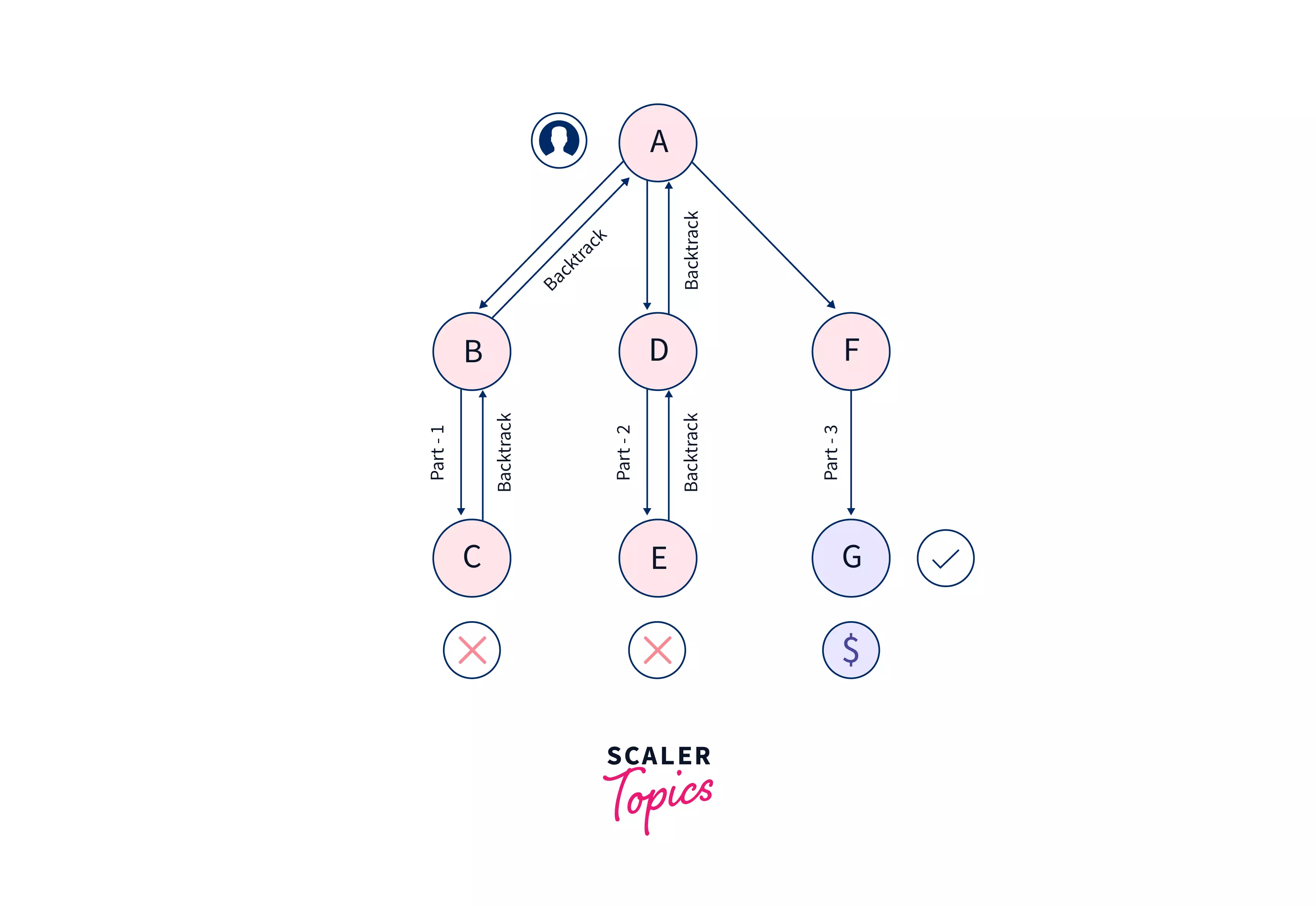
In the above example we see that —
- A is the starting point(or root) of our problem. So, initially we start from A and try to reach one of the possible solutions C, via B.
- Suppose, C turns out to be a non-feasible solution. Then, we again backtrack (go back) from C to A, via B. Check below, the actions taken by us
- Choose the 1st path: A–> B–> C => Not found our feasible solution => C–> B–> A (backtrack and move back to A again)
- After backtracking & Choosing the 2nd path: A–> D–> E => Not found our feasible solution => E–> D–> A (backtrack and move back to A again)
- Backtrack & Choose the 3rd path: A–> F–> G => Got our solution!
Summary:
- In this example,basically we started from the root node(A), and whenever we reached a point that was not an optimal solution (e.g. C or E), we backtracked (moved back) and again reached the root node. After that, we chose our next possible path to reach to our solution. We continued this till we were satisfied with our solution( Point G).
- Having considered the above approach of solving this problem, you may have noted that we traversed every possible combination before arriving at a feasible solution. Hence, we call backtracking a “brute-force algorithm.”.
- The above tree representation of a problem is called as a “space state tree”. It represents all possible states (solution or non-solution) of any given problem.
In backtracking we try to solve a subproblem, and if we don’t reach the desired solution, then undo whatever we did for solving that subproblem, and try solving another subproblem, till we find the best solution for that problem(if any).
Example
Problem Statement: Suppose you have 2 bikes ‘B1’ & ‘B2’. And 1 car ‘C’. Find all possible ways to arrange them. Constraint: Car should not be between bikes.
Expected output:
We have 4 possible ways :
B1 B2 C
B2 B1 C
C B1 B2
C B2 B1
Backtracking Algorithm: So, here we have a total of 3! = 6 possibilities. We will try all the possibilities and get the possible solutions. We recursively try all the possibilities.
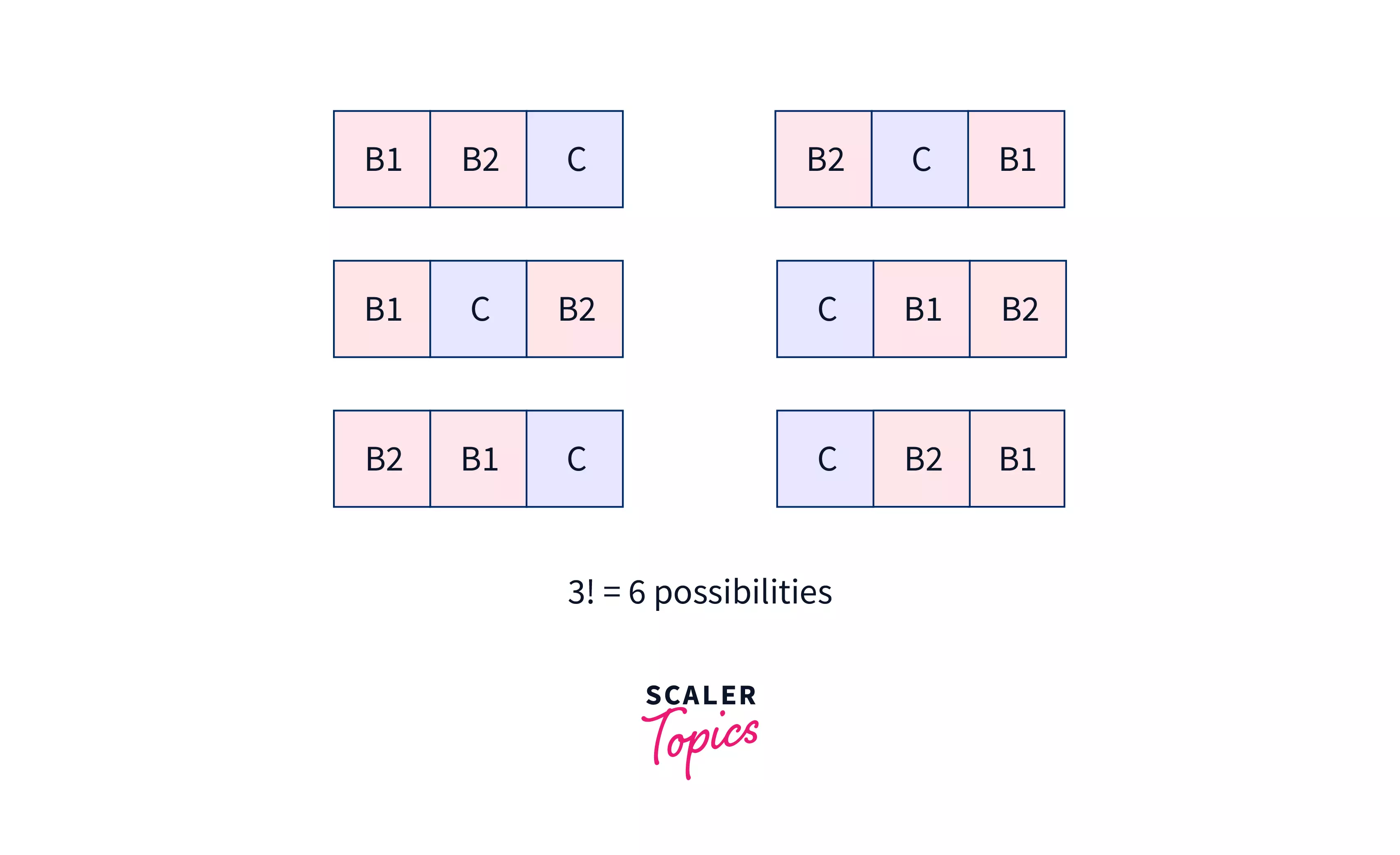
State space tree :
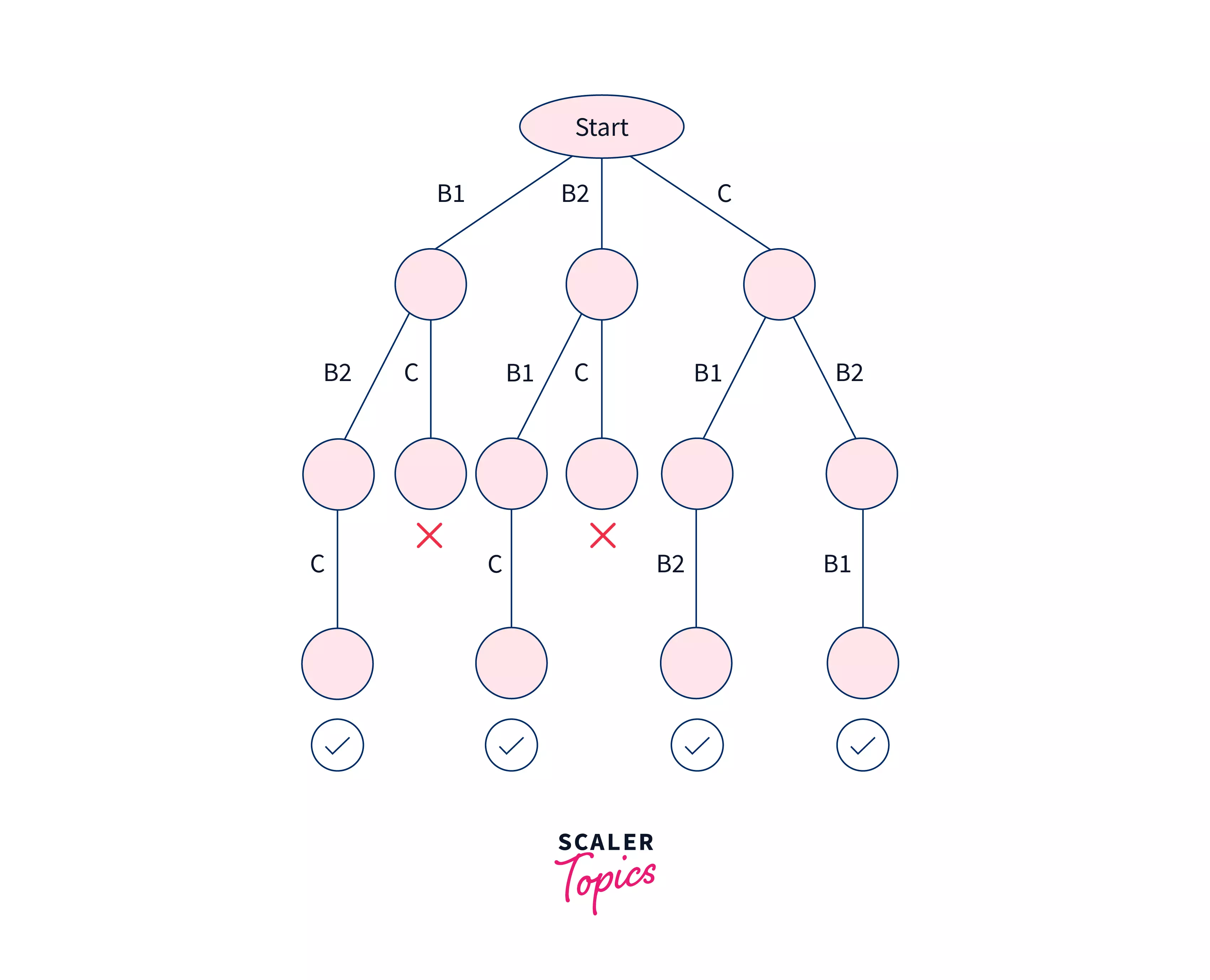
A space state tree is a tree representing all the possible states (solution or nonsolution) of the problem from the root as an initial state to the leaf as a terminal state.
In the above tree we see:
- We start from the Start Node. We traverse through: B1 -> B2 -> C => That is a possible solution since there is no car between bikes so we add it into our solutions list.
- Then we traverse our next possible path: B1 -> C => But we stop here because, a car is next to the bike and hence will be in the middle of the bikes in result. So, we backtrack to the starting point again, eliminating this result.
- Our next path is: B2 -> B1 -> C => This is one of our possible solutions, because here no car is between the bikes. Hence we add this to our solutions list.
- Next: B2 -> C => But we stop here because, a car is next to the bike. So, we backtrack to the starting point again, eliminating this result.
- Next: C -> B1 -> B2 => This is again one of our possible solutions, because here no car is between the bikes. Hence we add this to our solutions list.
- Next: C -> B2 -> B1 => This is again one of our possible solutions. Hence we add this to our solutions list too.
Final solutions list:
B1 B2 C
B2 B1 C
C B1 B2
C B2 B1
Let us see the algorithm for the same:
Algorithm:
Backtrack(z)
    if z is not a solution
        return false
    if z is a new solution
        add to list of solutions
    backtrack(expand z)
The algorithm states what we have done in our above problem.
- Start with the Start Node
- if the current point is a feasible solution, return true(success) and add it to the list of solutions.
- else if all paths are exhausted (i.e current point is an end point), return false(failure), since we have no feasible solution for the problem.
- else if current point is not an end point, backtrack and explore other points and repeat the above steps.
Advantages of Backtracking:
There are many advantages of backtracking. Few of them are
- Backtracking can almost solve any problems, due to its brute-force nature, although we use it to solve problems which have branching involved.
- Backtracking is an easy method to implement and contains fewer lines of code.
Disadvantages of Backtracking:
- More optimal algorithms for the given problem may exist.
- When the branching factor is high, it is very time-consuming
- Large space complexity because we are using recursion so function information is stored on stack.
Application of Backtracking
There are some problems that lend themselves best to backtracking solutions. Several of such problems follow
- To find all Hamiltonian Paths present in a graph.
- To solve the N Queen problem.
- Maze solving problem.
- The Knight’s tour problem.
- Binary Strings: generating all binary strings
- Generating k – ary Strings
- The Knapsack Problem
- Generalized Strings
- Graph Coloring Problem
Difference between Recursion and Backtracking
There is no major difference between these two in terms of their approach, except for what they do —
- Backtracking uses recursion to solve it’s problems. It does so by exploring all the possiblities of any problem, unless it finds the best and feasible solution to it.
- Recursion occurs when a function calls itself repeatedly to split a problem into smaller sub-problems, until it reaches the base case.
So, we may say recursion is a part of backtracking itself. However, there is no base case in backtracking to stop it. The backtracking mechanism will not stop as long as it finds an optimal solution to the problem.
Conclusion
Here we come to the end of the tutorial. It has provided you with a detailed understanding of recursion and backtracking as well as relevant examples. Let’s summarize what we have learned throughout the tutorial
- Recursion – why and how it is used.
- Base cases – Examples of recursion
- Backtracking – Details, why and how it is used
- Examples of backtracking
- Recursion vs Backtracking
- Advantages & disadvantages of recursion & backtracking
- Application of recursion & backtracking
Hope you enjoyed the tutorial. Happy coding!
Code with Precision! Enroll in Scaler Academy’s Online DSA Course and Master Efficient Algorithms.