A B+ Tree is simply an extended version of a B Tree, in which the values or pointers are stored at the leaf node level, making the various operations on it relatively easier.
The root node has a minimum of two children. Each node except root can have a maximum of m children and a minimum of $ m/2$ children. Each node can contain a maximum of m-1 keys and a minimum of ⌈m/2⌉ – 1 keys.
Scope
- This article describes the structure of a
B+ treealong with its properties in Data Structures. - It also discusses how different operations can be performed on it, along with code.
Takeaways
- Complexity of
B+ TreeTime complexity– $O(logn)$
Introduction to B+ Trees
A B+ Tree is simply a balanced binary search tree, in which all data is stored in the leaf nodes, while the internal nodes store just the indices. Each leaf is at the same height and all leaf nodes have links to the other leaf nodes. The root node always has a minimum of two children.
Everything keeps developing with time, our way of living, scientific inventions, be it literally anything! Such is the case with B trees!
The concept of B+ trees exists because of it being much more convenient, both in terms of operations on it, as well as efficiency.
We will discuss everything here in the next few sections, but a good knowledge of B trees is recommended before proceeding! Check out our B trees article here: B Tree
Once you’re done, we are ready to proceed! To have a more clear picture of how a B+ tree looks like, let’s now study its properties, one by one!
Properties of B+ Trees
- All data is stored in the
leaf nodes, while the internal nodes store just the indices. - Each leaf is at the same height.
- All leaf nodes have links to the other leaf nodes.
- The root node has a minimum of two children.
- Each node except root can have a maximum of m children and a minimum of
m/2children. - Each node can contain a maximum of m-1 keys and a minimum of
⌈m/2⌉ - 1keys.
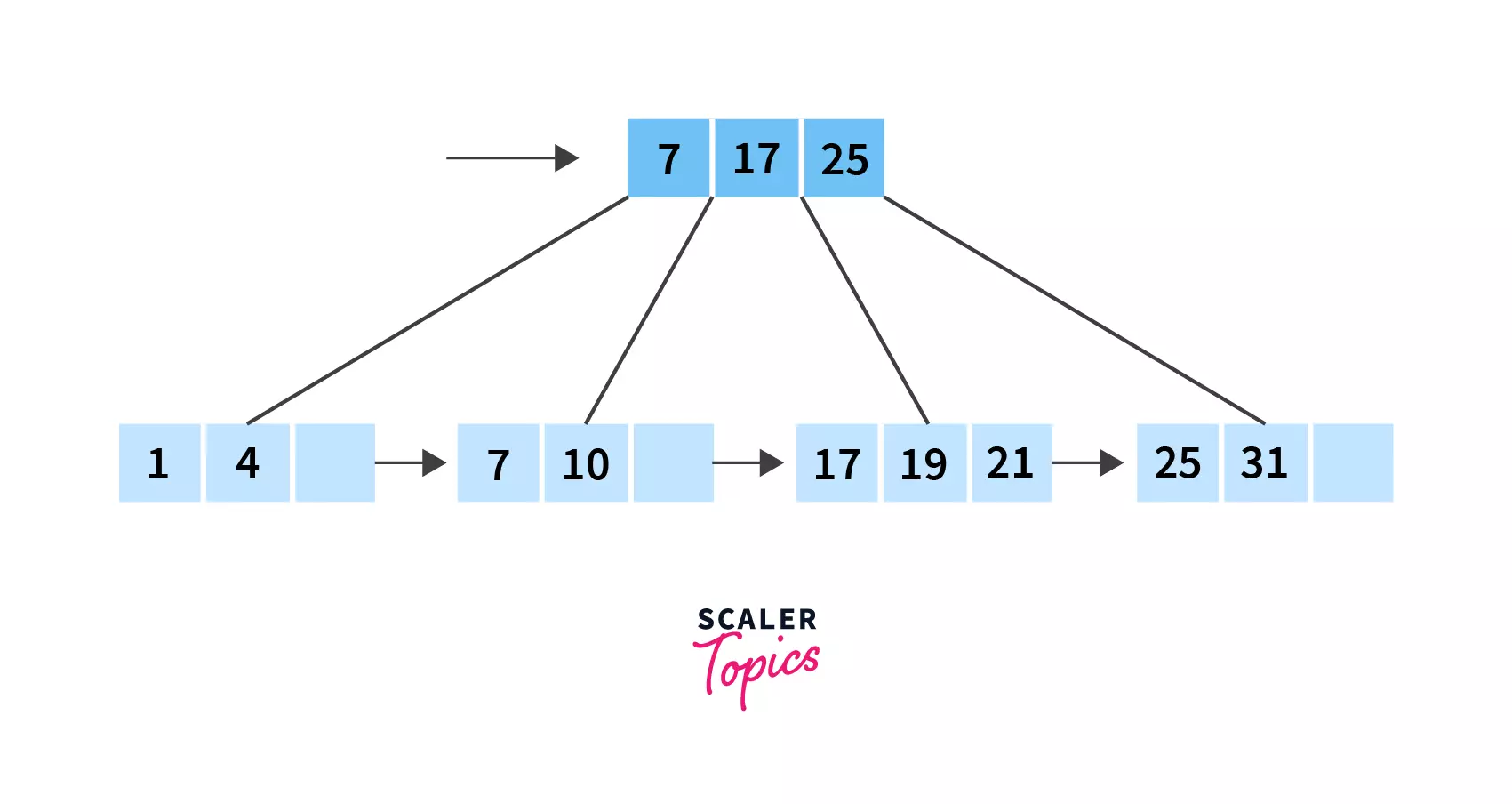
Go through all the above points again, you’ll see how all these properties make up a perfect B+ tree, in which all leaf nodes are at the same level, and how some of the values stored in the internal nodes act as pointers to the actual data present in the leaf nodes.
All these leaf nodes are linked to each other, making up a linked list. Also, if you’re wondering, this is why B+ trees are an important concept in DBMS!
We discussed that B+ trees are advanced and different from B trees. But how? We are about to find it out now!
Difference Between B Tree and B+ Tree
Now, we will have a look at how B+ Trees are different from B Trees, in detail:
| B Tree | B+ Tree |
|---|---|
| Data is stored in leaf as well as internal nodes | Data is stored only in leaf nodes. |
| Operations such as searching, insertion and deletion are comparatively slower. | Operations such as searching, insertion and deletion are comparatively faster. |
| No redundant search keys are present. | Redundant keys may be present. |
| Leaf nodes are not linked together. | Leaf nodes are linked together as a linked list. |
| They are not advantageous as compared to B+ trees, and hence, they aren’t used in DBMS. | They are advantageous as compared to B trees, and hence, because of their efficiency, they find their applications in DBMS. |
These are the points that differentiate B+ trees from B trees.
Also, do you remember that we earlier stated that operations on B+ trees are relatively easier? You must be wondering why! Let’s deep dive to find out that why we say that!
Operations on B+ Tree
Let’s look at the steps to perform the operations of insertion, deletion and searching a node in a B+ tree, along with an example each:
Insertion in B+ Tree
So first up is insertion. We will also learn how a B+ tree is created, here in this section! Let’s begin!
Before we look at the steps of insertion of a node, let’s understand the possible cases:
Case 1: The leaf node is not full
Insert the key into the leaf node in increasing order if the leaf isn’t full.
Case 2: The leaf node is full
Step 1: Insert the new node as a leaf node, in the increasing order. Now since the leaf node was already full, some balancing would be needed.
Step 2: Break the node at m/2th position.
Step 3: Add the m/2nd key to the parent node.
Step 4: In case the parent node is already full, just repeat the steps 2 and 3.
Reading the algorithm alone is not enough! Follow the example discussed below to understand how B+ trees are created and elements are inserted!
Example:
We need to use the following data to create the B+ Tree:1, 4, 7, 10, 17, 21, 31
We suppose the order(m) of the tree to be 4. The following facts can be deduced from this:
Max Children = 4
Min Children: m/2 = 2
Max Keys: m - 1 = 3
Min Keys: ⌈m/2⌉ - 1 = 1
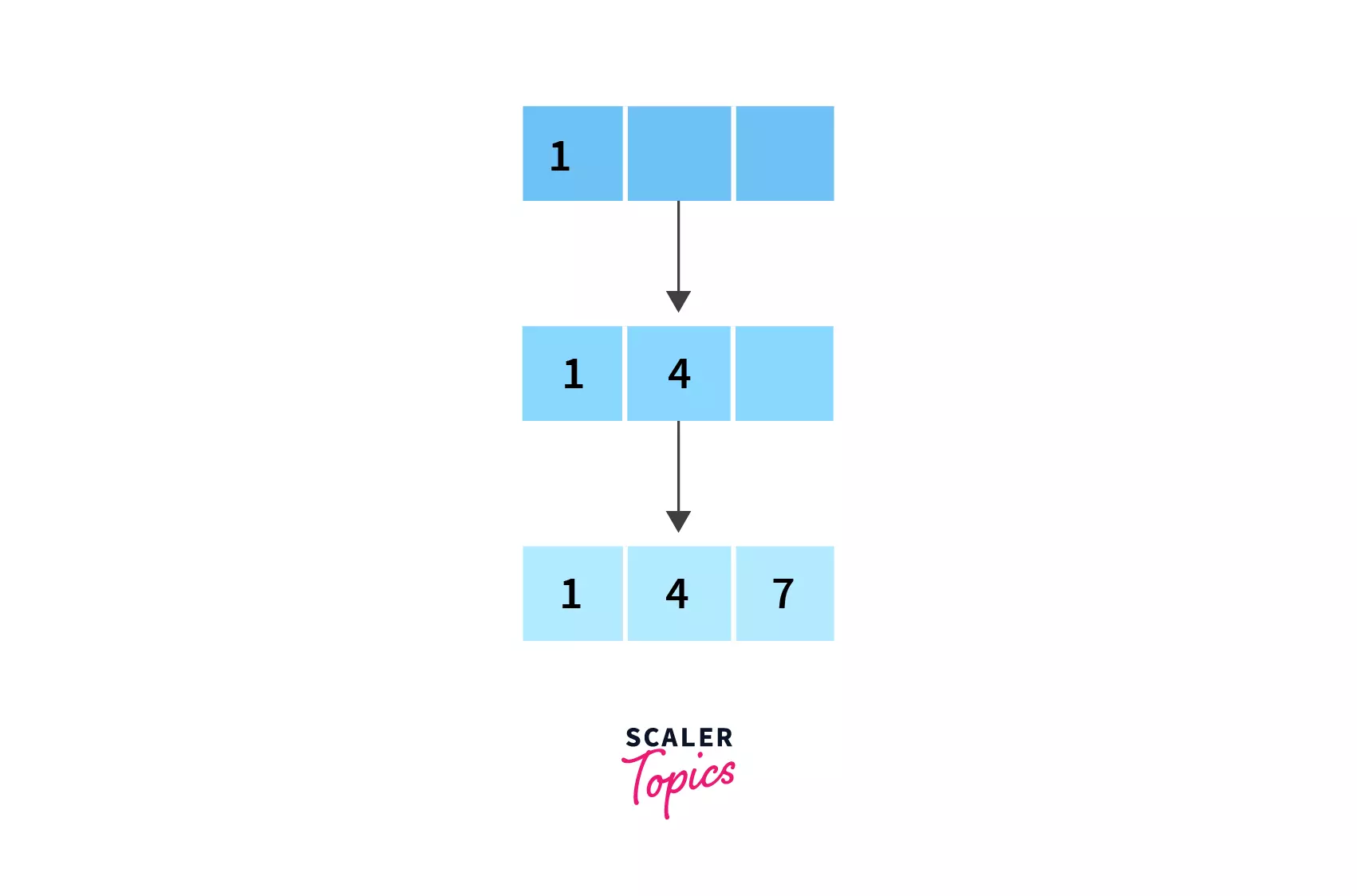
- Now, for our first step, let’s insert
1,4and7into the first node.
- The next element to be inserted is
10, but since there is no space in the current node (due to the maximum number of keys being3), we need to split it.
Here, we need to decide if we will be breaking the node at 4 or 7. Breaking the node at 4 will make the tree left biased, while breaking the node at 7 will make the tree right biased. Choose either of left biased, or right biased and follow it throughout the whole process!
- For this example, let’s choose the right biased tree. Hence, split the node at
7and move it up..
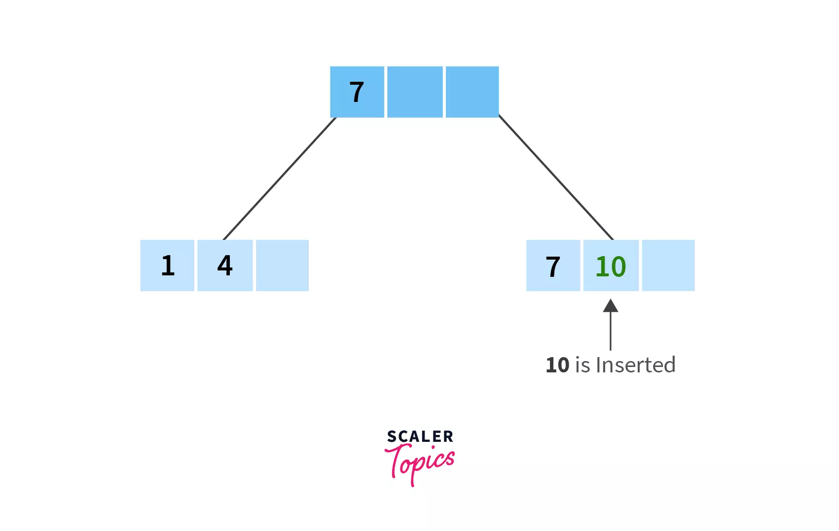
- Now we have split it into:
(i)1,4and a blank space (since the maximum number of keys in a node is3) and,
(ii)7and10.
We can now insert17into node(ii) as it would come after 10 in the ascending order.
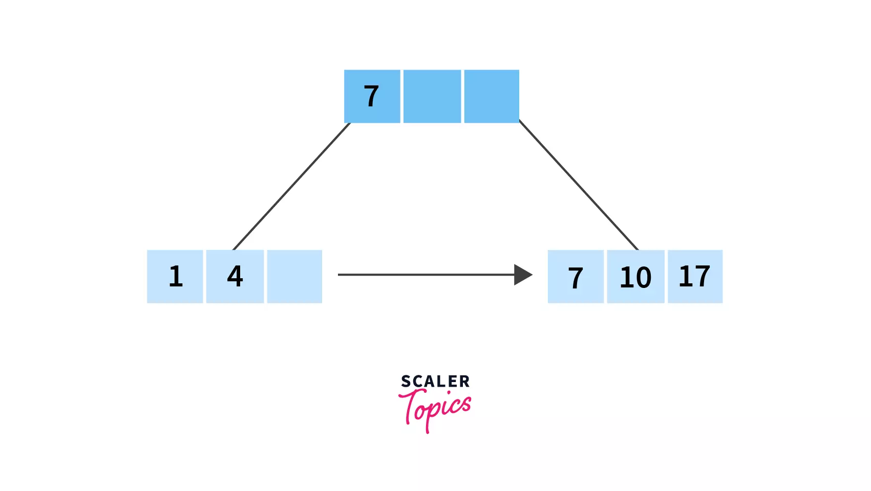
- Next to be inserted is
21, and ideally it should be placed after17. But since the node is full with3keys, we will have to split this node.
Now since we chose right biased after step2, we will split the node in this way:
(i)7, 10and a blank space
(ii)17, 21and a blank space.
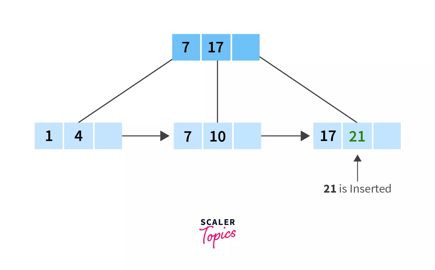
- Finally, let’s insert
31. It should be placed after21in the last leaf node. Which completes ourB+ tree!
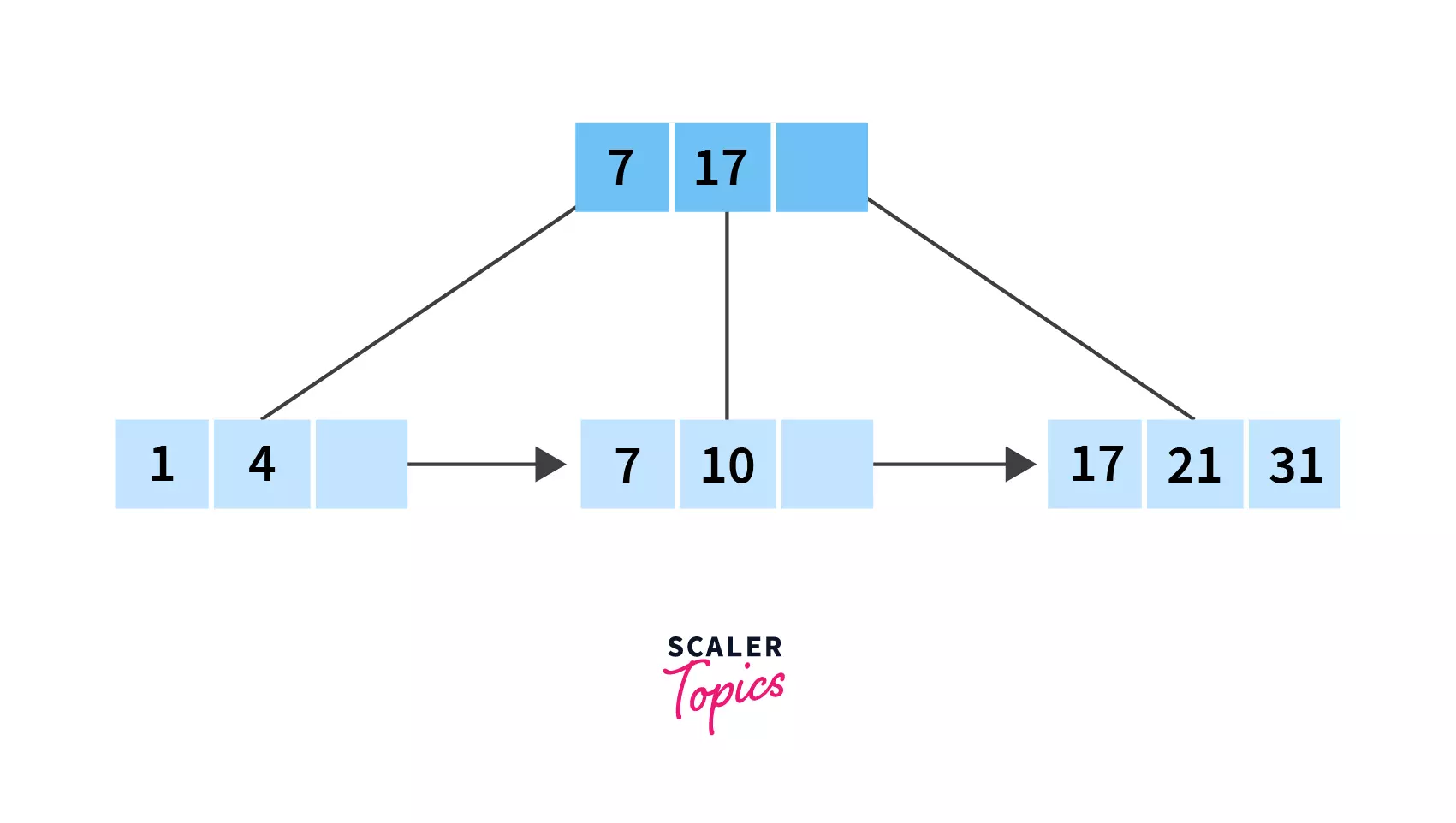
Note that all nodes have a minimum of 2 children, satisfying the facts that we deduced before we started implementing the B+ tree!
Deletion in B+ Tree
Now we know how a B+ tree is created and how nodes are inserted. But what if we have added a node that we don’t need anymore? Yes, we can delete it, but there are some rules to be followed!
Similar to insertion, we have two cases for deletion too!
Case 1: If the value to be deleted is present in the leaf node only
If the value to be deleted is present in the leaf node only, then just simply delete it!
Case 2: If the value to be deleted is present in the leaf node and has a pointer to it as well
Locate the node that you want to delete and remove it from the leaf node, but we also need to remove it from the index that points to this node. Remove the pointer and move the first value of the right child into the parent node.
That’s it!
Example:
Delete the value 21 from the following B+ Tree:
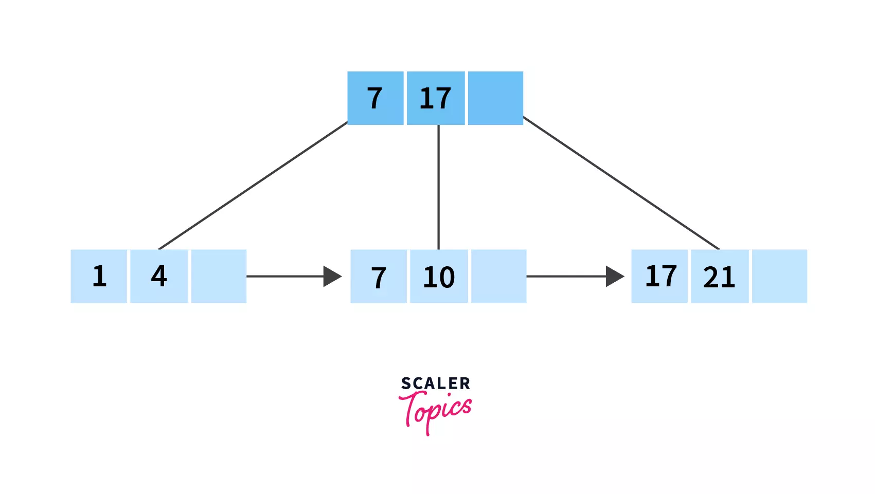
After Deletion:
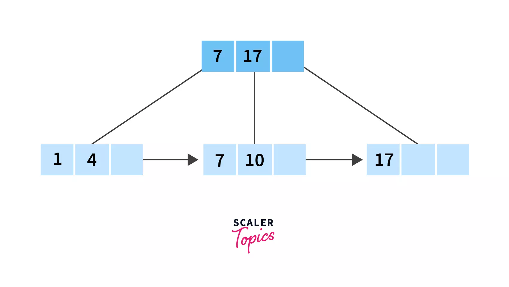
Since 21 is present only in the leaf node and deleting it wouldn’t invalidate the minimum number of keys (that is 1, as calculated), we can simply remove it!
Searching in B+ Tree
Searching in a B+ tree is really simple and efficient due to the fact that the leaf nodes, which v=contain the data are linked to each other by pointers, forming a linked list, as we discussed earlier too! This is why B+ tree finds its applications in DBMS too!
So, we are gonna understand the procedure for the same now, with the help of the following algorithm:
- Perform a binary search on the current node’s records.
- If a record matching the search key is discovered, return it.
- Report an unsuccessful search if the current node is a leaf node and the key is not found.
- Otherwise, go back to the beginning and repeat the process.
Example:
Search for 10 in the given B+ tree:
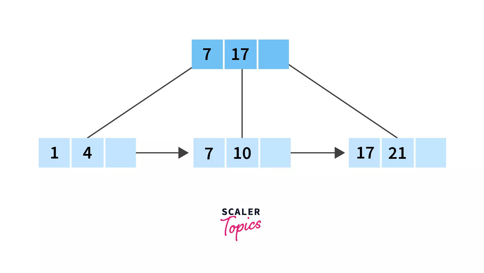
Firstly, we need to look at the indices. We have two of them, 7 and 17. Clearly 10 lies between them, so we need to search in the records between 7 and 17 which is leaf node number 2! And there is our required value, 10!
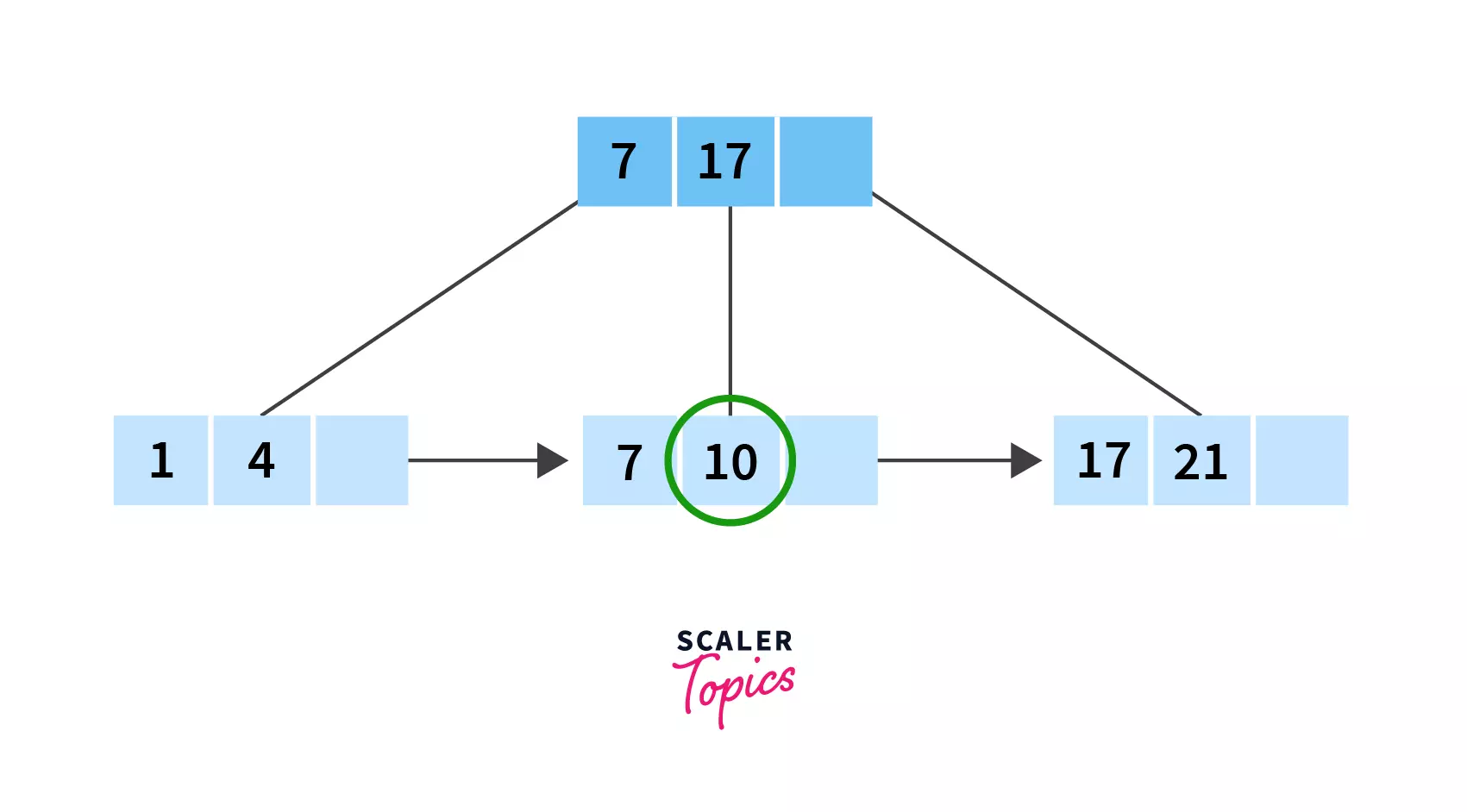
Pretty simple, isn’t it? Hopefully you’ve been able to understand how all these operations- insertion, deletion and searching work in the case of B+ trees. Also, you may have been able to see how these are easier as compared to operations performed on a B tree.
Advantages of B+ Tree
We have discussed a lot of times till now that how B+ trees are better than B trees and how they our useful in DBMS.
Let’s now summarise the advantages offered by B+ trees in points:
- Height of the
B+ treeis always balanced and is comparitively lesser thanB tree. - It takes equal number of disk accesses to fetch records.
- Keys are used for indexing.
- Because the data is only stored on the leaf nodes, search queries are faster.
- Data stored in a
B+ treecan be accesssed both sequentially and directly.
Applications of B+ Tree
B+ trees have many applications. We will state some of them below:
B+ treesin DBMS plays a useful role by supporting equality and range search.- It also facilitates database indexing in DBMS.
- Another advantage is multilevel indexing.
B+ Tree Operation Code in Python
Finally, it’s now time to code! How are B+ trees implemented in code? Let’s find out together:
    class Node(object):

    def _init_(self, curorder):

        self.curorder = curorder
        self.key = []
        self.value = []
        self.leaf = True
Each node stores keys and values. The variable curorder stores the maximum number of keys that each given node can store.
    def add(self, key, value):
        if not self.key:
            self.key.append(key)
            self.value.append([value])
            return None
The above function adds a key-value pair to the node by just inserting the key-value pair if the node is empty.
Now, if the new key is the same as an existing key, it should be added to the list of values. Let’s do that next:
    for i, val in enumerate(self.key):
            if key == val:
                self.value[i].append(value)
                break
Also, if the new key is smaller than the old one, place it to the left of the old one:
        elif key < val:
                self.key = self.key[:i] + [key] + self.key[i:]
                self.value = self.value[:i] + [[value]] + self.value[i:]
                break
And finally, if the new key is larger than all the others, place it to the right of the other existing keys:
            elif i + 1 == len(self.key):
                self.key.append(key)
                self.value.append([value])
As we discussed in the algorithm, sthe following function splits the node into two parts, which are then stored as child nodes:
    def split(self):
        l = Node(self.curorder)
        r = Node(self.curorder)
        mid = self.curorder // 2

        l.key = self.key[:mid]
        l.value = self.value[:mid]

        r.key = self.key[mid:]
        r.value = self.value[mid:]
Let’s set the parent key to the left-most key of the right child node when the node is split:
    self.key = [r.key[0]]
        self.value = [l, r]
        self.leaf = False

    def is_full(self):
        return len(self.key) == self.curorder

    def show(self, counter=0):
        print(counter, str(self.key))

        if not self.leaf:
            for val in self.value:
                val.show(counter + 1)
Now, the following is a B+ tree object, consisting of nodes. When a node reaches full capacity, it will automatically split into two. A key will ‘float’ upwards and be put into the parent node to act as a pivot when a split occurs.
The attribute “curorder” is the maximum number of keys that each node can store.
    class MakeTree(object):
    def _init_(self, curorder=8):
        self.root = Node(curorder)
The below function returns the index where the key should be placed as well as a list of values at that position, for a given node and key…
    def _find(self, node, key):
        for i, val in enumerate(node.key):
            if key < val:
                return node.value[i], i

        return node.value[i + 1], i + 1
Now, extract a pivot from the child node to be inserted into the parent’s keys for a parent and child node. Put the values from the child into the parent’s values:
    def _merge(self, parent, child, index):
        parent.value.pop(index)
        pivot = child.key[0]

        for i, val in enumerate(parent.key):
            if pivot < val:
                parent.key = parent.key[:i] + [pivot] + parent.key[i:]
                parent.value = parent.value[:i] + child.value + parent.value[i:]
                break

            elif i + 1 == len(parent.key):
                parent.key += [pivot]
                parent.value += child.value
                break
Then, we insert a key-value pair when reaching a leaf node.
Until we reach a leaf node, we keep traversing the tree, and if the leaf node is full, we split the leaf node into two!
    def insert(self, key, value):
        parent = None
        child = self.root

        while not child.leaf:
            parent = child
            child, index = self._find(child, key)

        child.add(key, value)

        if child.is_full():
            child.split()
When a leaf node is split, it is made up of two leaf nodes and an internal node. These will have to be re-inserted into the tree.
        if parent and not parent.is_full():
                self._merge(parent, child, index)

    def retrieve(self, key):
        child = self.root

        while not child.leaf:
            child, index = self._find(child, key)

        for i, val in enumerate(child.key):
            if key == val:
                return child.value[i]

        return None

    def show(self):
        self.root.show()

    def demo_node():
        print('Initializing Tree')
        node = Node(curorder=4)

    print('\nInserting key a')
    node.add('a', 'Scaler1')
    print('Is node full?', node.is_full())
    node.show()

    print('\nInserting key b, c, d')
    node.add('b', 'Scaler2')
    node.add('c', 'Scaler3')
    node.add('d', 'Scaler4')
    print('Is node full?', node.is_full())
    node.show()

    print('\nSplitting node')
    node.split()
    node.show()

    def demo_tree():
        print('Initializing B+ tree')
        tree = MakeTree(curorder=4)

    print('\nB+ tree with 1 val')
    tree.insert('a', 'Scaler1')
    tree.show()

    print('\nB+ tree with 2 vals')
    tree.insert('b', 'Scaler2')
    tree.show()

    print('\nB+ tree with 3 vals')
    tree.insert('c', 'Scaler4')
    tree.show()

    print('\nB+ tree with 4 vals')
    tree.insert('d', 'Scaler5')
    tree.show()

    print('\nB+ tree with 5 vals')
    tree.insert('e', 'Scaler6')
    tree.show()

    print('\nB+ tree with 6 vals')
    tree.insert('f', 'Scaler7')
    tree.show()

    print('\nRetrieving value with key e')
    print(tree.retrieve('e'))

    if _name_ == '_main_':
        demo_node()
        print('\n')
        demo_tree()
So here we are folks! All done and dusted! Congratulations! You’re now thorough with all the concepts of a B+ tree. Let’s conclude and see what all we studied!
Conclusion
- Firstly, we developed a brief understanding of what a
B+ Treeis, by means of the definition and properties. - We saw what points differentiate
B+ treesfromB- trees. - We looked at the steps for performing different operations on B+ trees,
i.e.insertion, deletion and searching. - And finally, we looked at what advantages
B+ treesoffer, the applications, along with their implementation with code.
Dive into the World of Efficient Coding – Enroll in Scaler Academy‘s DSA Course Today and Learn from Industry Experts!
